In this article, I explain the intuition behind an image processing technique called Poisson Blending. This technique is an image processing operator that allows the user to insert one image into another, without introducing any visually unappealing seams. Furthermore, this technique also makes sure that the color of the inserted image is also shifted, so that the inserted object feels as if it is part of the environment of the target image. So a bright object copy-and-pasted into a rather dark image, will have its color shifted to a darker color. The reason “Poisson Blending” achieves a more realistic looking composition than naively pasting two similarity colored images together is because the human visual system is more sensitive to contrast than intensity values. Note that the code part discussed here is in Python but can be translated to any language.

Gradient Preserving property
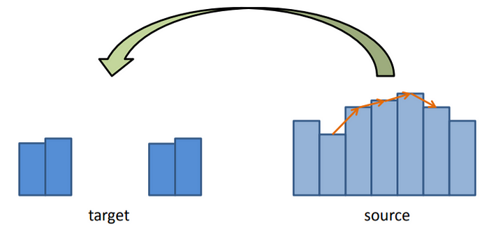
The main problem in doing some basic gradient based approaches is that we are unable to preserve the gradient in this process as shown below:-
Basic Idea
This whole algorithm actually boils down to a very simple idea. To get at this, let’s first try to define more carefully what we’d like to accomplish when we blend two images together. Call the image we’re changing Image A and the image we’re cutting out and pasting Image B:-

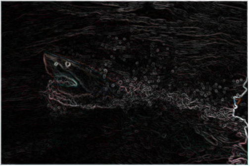
It would be nice if we could allow the colors in Image B to change when we pasted it on, but to somehow keep all of the “details” of Image B intact. Some details we’d like to preserve would be all of the edges, corners, transitions, etc in image B. Thus we use image gradient. The image gradient is just a mathematical way of describing how the image pixels change relative to the pixels around them (it is essentially the difference of a pixel and its neighbors). And a relative descriptor is just what we’re looking for, since the disagreement between image A and image B that makes them just out against each other is the absolute magnitude of their colors. Hence, the goal of Poisson Image Editing stated with a bit more rigor is: allow for the tweaking of absolute information of image B (colors), but preserve the relative information (image gradient) of image B as much as possible after it’s pasted. Below is the image gradient of the shark we’re trying to paste, so you can get an idea of what that relative information might look like:-
Given alone, the image gradient is under-constrained. As an analogy, consider I told you I wanted you to trace a path on a piece of paper, and I told you “first trace two inches, then turn 30 degrees clockwise, then trace 3 inches, etc”, but I didn’t tell you a starting position or any specific points on the path. Then the curve you trace out could start anywhere and be at any rotational orientation and still satisfy the conditions I told you. The relative information contained in the image gradient is the same way. We need to fix RGB values of some specific pixels to get a solution to our problem. This gives us an awesome opportunity to make image B more like image A. What we do is fix the pixels on the boundary of image B to be equal to the pixels on image A where B resides, and then solve for the rest of the pixels on the interior of image B that preserve the original gradient of image B. That’s it! In the next section I will give more specific equations for doing this and give even more intuition for how this works, but hopefully now you at least see what needs to be done.
Poisson Blending Algorithm
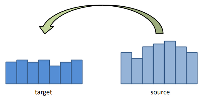
Given that people often care much more about the gradient of an image than the overall intensity. Therefore, we compute information about the gradient for each pixel in that part of the source image, and then apply the same gradient in the target image. The result is that each “transplanted” pixel on the target image has a gradient that is the same as the gradient of the corresponding pixel on the source image, but still have all the features of the source image. The main logic is -“A good blend should preserve gradients of source region without changing the background”. We treat pixels as variables to be solved. We minimize squared difference between gradients of foreground region and gradients of target region keeping the background pixels constant.


Prior to running the algorithm, a mask needs to be manually generated that indicates the overlapping region between the source (image being inserted) and the target (image the source is being inserted into).
The mask and source images are first padded so that they are the same size as the target image. Next, they are translated using parameterized row/column offsets. If the valid pixels in the mask are on the edge of the source image, a 1 pixel symmetric buffer is added to all 3 images to make processing easier. This 1 pixel buffer is then cropped off later from the result.
A linear system of equations is required to compute the resulting image from the source and target gradients. This system is represented by AX=B, where A is the sparse coefficients matrix, X is the output image, and B is the desired gradient matrix. The size of sparse matrix A is NxN, where N is target image rows multiplied by target image columns.
For pixels outside the masked region, the output image pixel is simply the same as the target image. For these pixels, the row in the sparse matrix A is simply the same as the identity matrix. Also for these pixels, the corresponding value in the desired pixel gradient matrix B are also the same pixel value as the target image. For pixels inside the masked region, the output image pixel x at (row, col) depends on its neighbors according to the following equation:

For these pixels inside the masked region, the row in the sparse matrix then contains these coefficients at the corresponding indices. The value of the desired pixel gradient is in matrix B and changes according to Mixing Gradients.
Approach
The image blending problem is phrased as a least-squares problem, which requires solving AX = B for every pixel under the mask.
We have a mask which has the same size as both the source and target images. The mask’s values are either 0 or 1. In our final image, if the mask’s value is 0, we want to just take the target’s pixel value at that point. If it is 1, we want to set up a linear equation such that the gradient for a given pixel is the same in both the source and final images.
We go through the entire image and create a vector with one entry for each pixel which takes the actual values of either the target image, if the mask was 0 at that point, or the gradient value from the source if the mask was 1 at that point. Once we have the coefficient matrix A and B, we can find our output image.
Matrix A and B generation

Now before all this we need to learn to make “A” using sparse matrices approach. The sparse matrix is made using “scipy.sparse.lil_matrix((target_height, target_height))”(call it ‘fl’). We then set its diagonals using fl.setdiag(-1, -1), fl.setdiag(4), fl.setdiag(-1, 1). We then generate the matrix A as “A = scipy.sparse.block_diag([fl] * target_height).tolil()” and set its diagonal too using A.setdiag(-1, 1*target_height), A.setdiag(-1, -1*target_height). The creation of this sparse matrix was also optimized by using tocsc() function. After all this we iterate through all the points in the target width and height. We define each pixel position as “pix = i+j*target_height” and set A[pix,pix] = 1 and all the 4 neighbours as 0. We then save it using compressed column format(tocsc()) as told before.
B represents the desired output gradient and values. A is same across all color channels hence we create it only once, but we calculate three different B column vectors: one for each color channel. For implementation, we first flatten all the three images i.e. source, target and mask. For source and target we need to take care about cropping to the size of target width and height. Then for each channel, we use the dot product of this flattened source and filter matrix generated earlier. We also use the flattened mask to generate a boolean which is then used by flattened target to give us the desired B matrix. We finally use these 2 matrices A and B to solve for the final image using ‘spsolve’ function and scaling values accordingly.
Discrete Solution
Let me now present the system of equations that solves the problem. Let’s call the image which we’re pasting on A (as before), the image which we’re pasting B (as before), and the new image to be pasted H (where H should be some improved version of B that blends in with A better). First the easy part: the boundary constraints. We said before the pixels on H’s boundary should be exactly the same as the pixels of A on that boundary, so that we can match those pixels on the outside of the selection and blend them inwards. In math speak:-

So we already know the exact solution to all pixels on the boundary of H (which is also the boundary of B). Now we need to solve for the pixels in the interior of H. We want the gradient of the pixels on the interior of H to equal the gradient of the pixels on the interior of B. A simple way to define a gradient of an image at a spot is the sum of the differences between that pixel and all of its neighbors:-

If one of the neighbors happens to be a boundary pixel, then its value is fixed. If one of the neighbors happens to be out of bounds of the selection, then it should be excluded. This is summarized for all cases for every point in H by the following difference equation (lifted from the paper and rearranged in a way that I think makes more sense):-

where (x, y) is the location of the point of interest on the 2D grid, “N” is the number of valid neighbors the pixel actually has within the selection region including the boundary (less than or equal to 4), “Omega” is the selection area of B and H excluding the boundary, “partial Omega” is the boundary of the selection area, and (dx, dy) are the possible neighbor locations that range over {(-1, 0), (1, 0), (0, -1), (0, 1)} (this accounts for the 4 possible neighbors of each point). This looks like a mess but it really isn’t, so let me break down this equation in English:-
- The left hand side of the equation is computing the spatial gradient of the unknown point H(x, y) by taking summing the difference between H(x, y) and all of its N neighbors. Each difference that goes into the gradient has the form H(x, y) — other(x’, y’), where (x’, y’) is the position of a neighbor. The first sum on the left hand side represents the difference of H(x, y) with other H(x’, y’) points that are on the interior of the selection (Omega). The second term represents the difference of H(x, y) with border points, which are fixed at the value of the image that we’re pasting onto, A, which is why we have to treat them separately (they do not vary and we do not solve for them).
- The right hand side of the equation is simply the gradient of image B at (x, y), which we would like to match with the gradient of our new image H at (x, y). Hence the equality.
- Note that for color images, these equations are set up and solved for the Red, Green, and Blue channels independently.
Hopefully this makes some sense. If it doesn’t, just remember the basic idea: we’re trying to solve for a new image H that matches the background of A better, and the border of this image H matches up with A exactly, while the difference between adjacent points of H matches up with the difference of the corresponding adjacent points in B.

